Universe Viewer

Universe Viewer is an interactive software for the visualization and geodesic analysis of high-redshift astronomical objects.

It allows for the production of a conformal map of cosmological structures, more specifically quasars, by taking into account the curvature of the universe. Based on concepts from astronomy and general relativity, it is designed to be a working tool for research in cosmology, facilitating the identification of large-scale structures in comoving space or in a reference space.

This project is based on the concepts developed in the publication Framework for cosmography at high redshift, by R. Triay, L. Spinelli, R. Lafaye.

It is free software, and its source code is available on its GitHub page.

This web version of the software was ported from the the Java version (which is no longer maintained today), with the help of artificial intelligence to speed up the tedious sequences of converting code from Java / Swing / JOGL to JavaScript / Vue.js / Vuetify / Three.js.

I particularly thank Pr. Roland Triay for his help during the design of the Java version of the software, created as part of my Master's training during a research study project (TER), carried out in tandem with Julie Fontaine, in 2008.

Even older versions of a similar software existed, in Fortran and C, based on the same research publication, but they suffered from portability issues.

Map Projection of Objects

The Framework for cosmography at high redshift presents a framework for projecting the studied objects onto a plane, depending on the chosen cosmological parameters and the viewpoint.

These objects are defined by three main characteristics:

• the right ascension, the first term associated with the equatorial coordinate system, it is the azimuth, the equivalent on the celestial sphere of terrestrial longitude,
• the declination, the second term, which measures the angle of an object from the celestial equator, it is the elevation, the equivalent of terrestrial latitude,
• and the object’s redshift, a relativistic effect that allows its distance from the observer to be inferred.

It is therefore from this data that the objects are represented on screen. Initially, the projection onto the reference space was developed for the case of a positive curvature of the universe, then this work was generalized to negative curvature. The calculations were finally extended for representation in comoving space, which abstracts from the expansion of the universe.

Calculation of Comoving Distance

The comoving distance (dimensionless) is denoted $\tau$, it depends on the redshift z of the object concerned and is calculated as follows:

$$\tau (z)={\int }_{(1+z{)}^{-1}}^1\frac{da}{\sqrt{P(a)}}$$

where:

$$P(a)={\lambda }_0{a}^4-{\kappa }_0{a}^2+{\mathrm{\Omega }}_{0}a+{\alpha }_0$$$$P(1)=1$$

${\lambda }_0$, ${\kappa }_0$, ${\alpha }_0$, ${\mathrm{\Omega }}_0$ are the cosmological parameters:

• ${\lambda }_0$, a cosmological constant standing for vacuum energy,
• ${\kappa }_0$, the curvature parameter, defining the global universe geometry,
• ${\alpha }_0$, accounts for the presence of cosmic microwave background photons as sources of gravity,
• ${\mathrm{\Omega }}_0$, the matter density parameter,

and a represents the cosmological scale factor. For an observed object with a redshift z, it is equal to:

$$a(t)=\frac{1}{1+z}$$

This scale factor describes the state of expansion of the Universe at the moment the light was emitted. Today, we have $a_0=1$.

Normalization of Comoving Distance in Curved Geometry

When the comoving space is not flat (${\kappa }_0\ne 0$), the angular distance is introduced:

$$\hat{\tau }=\tau \sqrt{|{\kappa }_0|}\text{with}{\kappa }_0\ne 0$$

This variable naturally appears in the non-zero curvature spatial metric:

$$\{\begin{array}{ll}R=\frac{\sin (\hat{\tau })}{\sqrt{{\kappa }_0}}& {\kappa }_0>0\\ R=\frac{\sinh (\hat{\tau })}{\sqrt{-{\kappa }_0}}& {\kappa }_0<0\end{array}$$

In the specific case of flat space (${\kappa }_0=0$):

$$R=\tau$$

R is used to place points in the curved geometry.

Calculation of the Projection onto the Observation Plane

Each cosmological object is represented by a 4D vector in the homogeneous spacetime of the model:

$$\overrightarrow{X}=(x,y,z,t)$$

The first three coordinates (x, y, z) represent the spatial position of the object in the 3D embedding space corresponding to the chosen geometry (spherical if ${\kappa }_0$ > 0, hyperbolic if ${\kappa }_0$ < 0, or flat if ${\kappa }_0$ = 0).
The fourth coordinate t represents the conformal temporal component (associated with the comoving distance $\tau$) in the homogeneous spacetime.

The x, y and z coordinates are calculated as follows:

$$x=R\cos (De{c}_{obj})\cos (R{A}_{obj})$$$$y=R\cos (De{c}_{obj})\sin (R{A}_{obj})$$$$z=R\sin (De{c}_{obj})$$

where $R{A}_{obj}$ and $De{c}_{obj}$ are the right ascension and the declination of the objet.

In reference space, $t=\tau$, and in comoving space:

$$t=\tau \sqrt{|{\kappa }_0|}$$

The 2D display requires projecting this 4D vector onto an image plane, which represents the plane of the sky according to the viewpoint.

Construction of the Local Observation Basis

The user defines their orientation in the universe using three angles:

• RA1, the right ascension (azimuth),
• Dec1, the declination (elevation),
• Beta, the rotation around the line of sight (roll).

From these angles, three orthonormal vectors are constructed in the 3D Euclidean space:

• $\overrightarrow{P_1}$: direction of gaze (center of the projection),
• $\overrightarrow{P_2}$: local horizontal direction,
• $\overrightarrow{P_3}$: local vertical direction.

These three vectors form a spatial orthonormal basis. In the 4D spacetime of the model, this basis becomes:

$${\overrightarrow{E}}_1=\left(\begin{array}{c}\overrightarrow{P_1}\\ 0\end{array}\right)\text{,}{\overrightarrow{E}}_2=\left(\begin{array}{c}\overrightarrow{P_2}\\ 0\end{array}\right)\text{,}{\overrightarrow{E}}_3=\left(\begin{array}{c}\overrightarrow{P_3}\\ 0\end{array}\right)$$

The fourth basis vector is defined as:

$${\overrightarrow{E}}_0=\left(\begin{array}{c}\overrightarrow{0}\\ s\end{array}\right)$$

where:

$$s=\{\begin{array}{ll}1& \text{in the reference space}\\ \sqrt{|{\kappa }_0|}& \text{in the comoving space}\end{array}$$

This vector encodes the temporal component of the frame. Its normalization depends on the chosen space (reference or comoving), as this ensures that the projections respect the model's metric.

Projection onto the Image Plane

For an object whose 4D vector is $\overrightarrow{X}$, its projected coordinates on the 2D plane are:

$$x_{\text{proj}}=\overrightarrow{X}\cdot {\overrightarrow{E}}_1=X_x{E}_{1x}+X_y{E}_{1y}+X_z{E}_{1z}+X_t{E}_{1t}$$$$y_{\text{proj}}=\overrightarrow{X}\cdot {\overrightarrow{E}}_2=X_x{E}_{2x}+X_y{E}_{2y}+X_z{E}_{2z}+X_t{E}_{2t}$$

Examples of Projections

Hewitt & Burbidge QSO Catalog

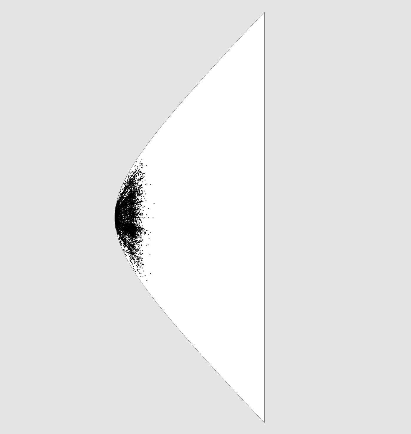
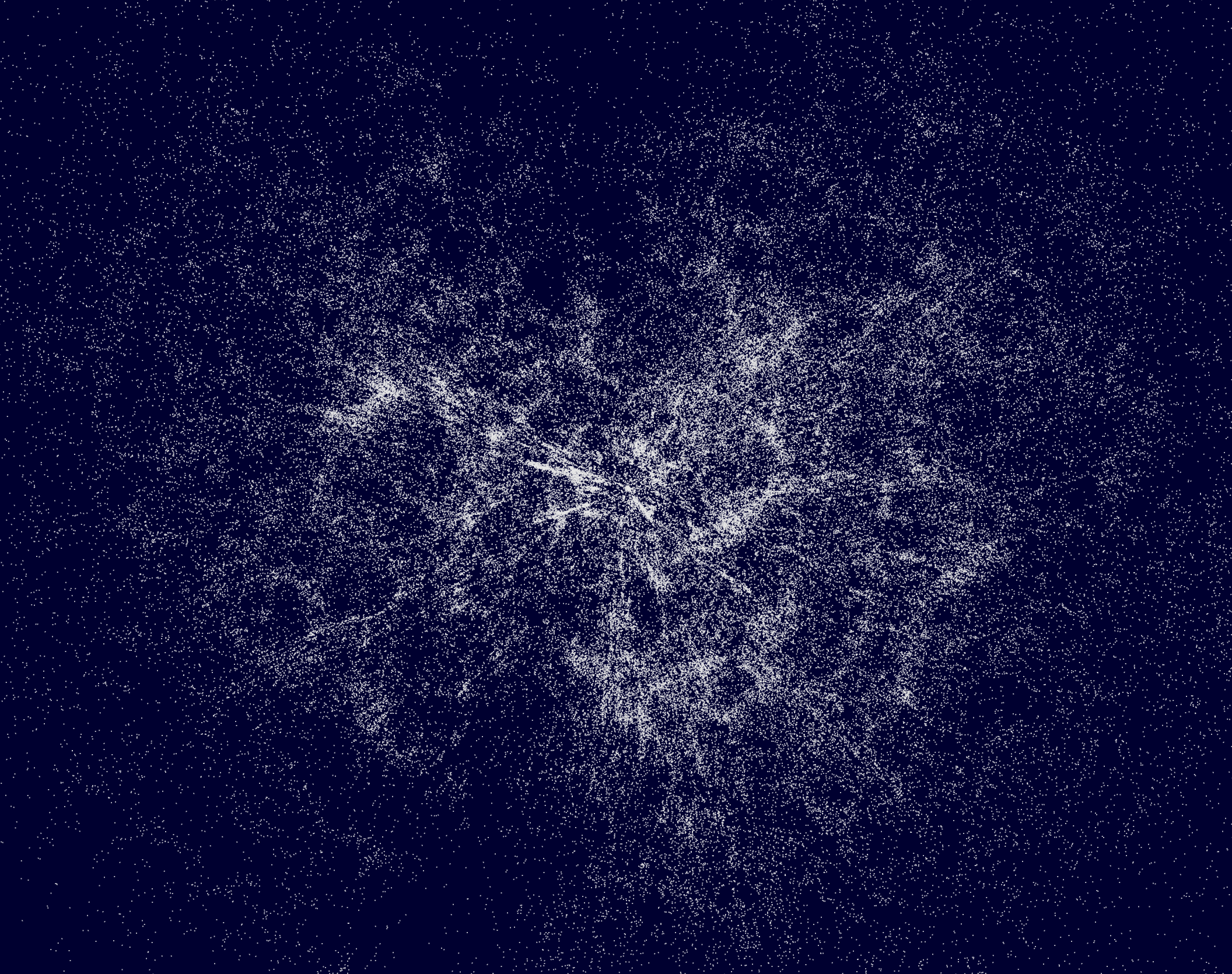
Here are some projections obtained on the Hewitt & Burbidge quasar catalog, composed of 7,236 objects.

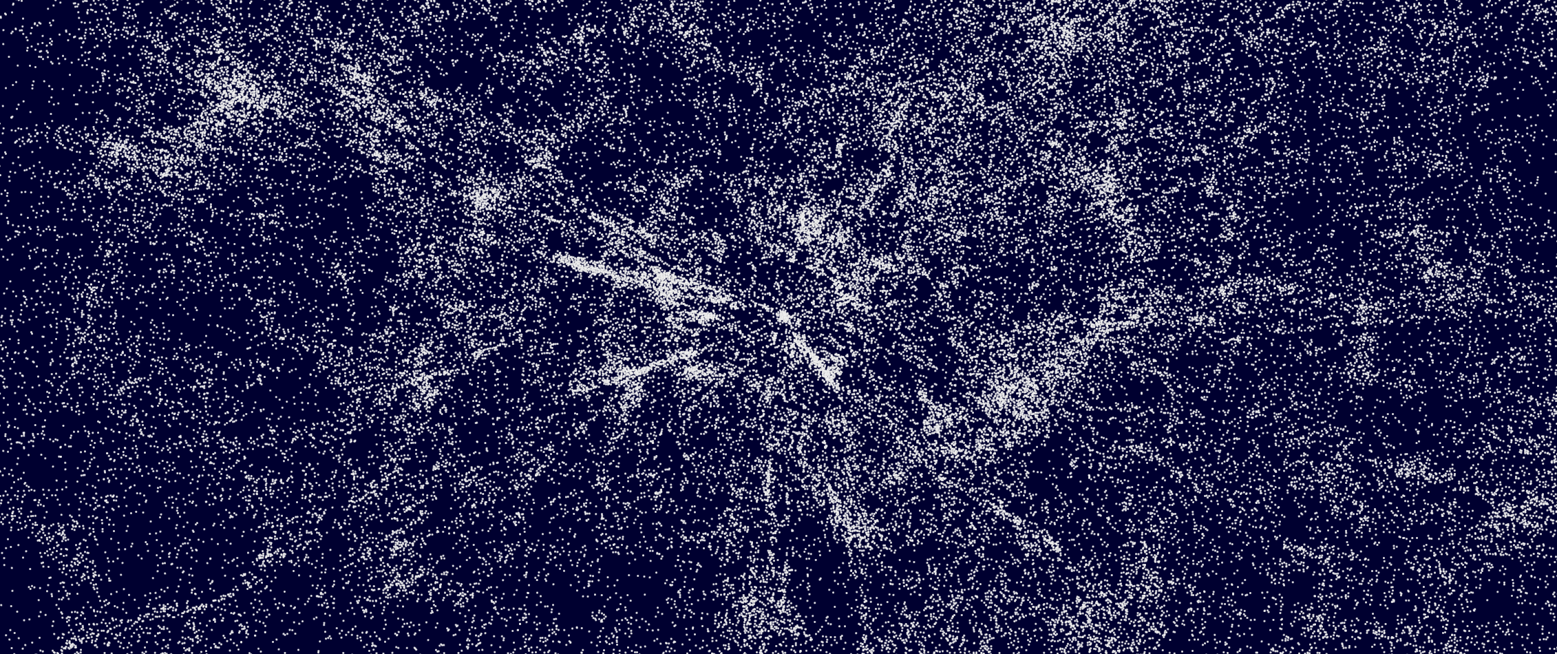
The blue area represents the visible universe, the gray line surrounding it is the cosmological horizon.

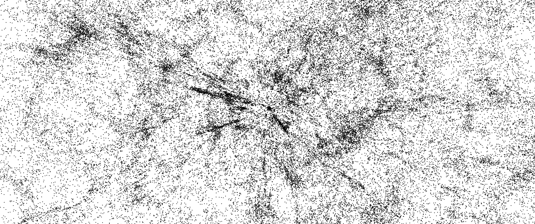
The white area represents the visible universe, the black line surrounding it is the cosmological horizon.

Front view, positive curvature

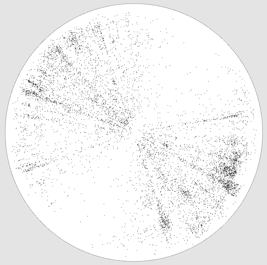Our galaxy is at the center.

Edge view, positive curvature

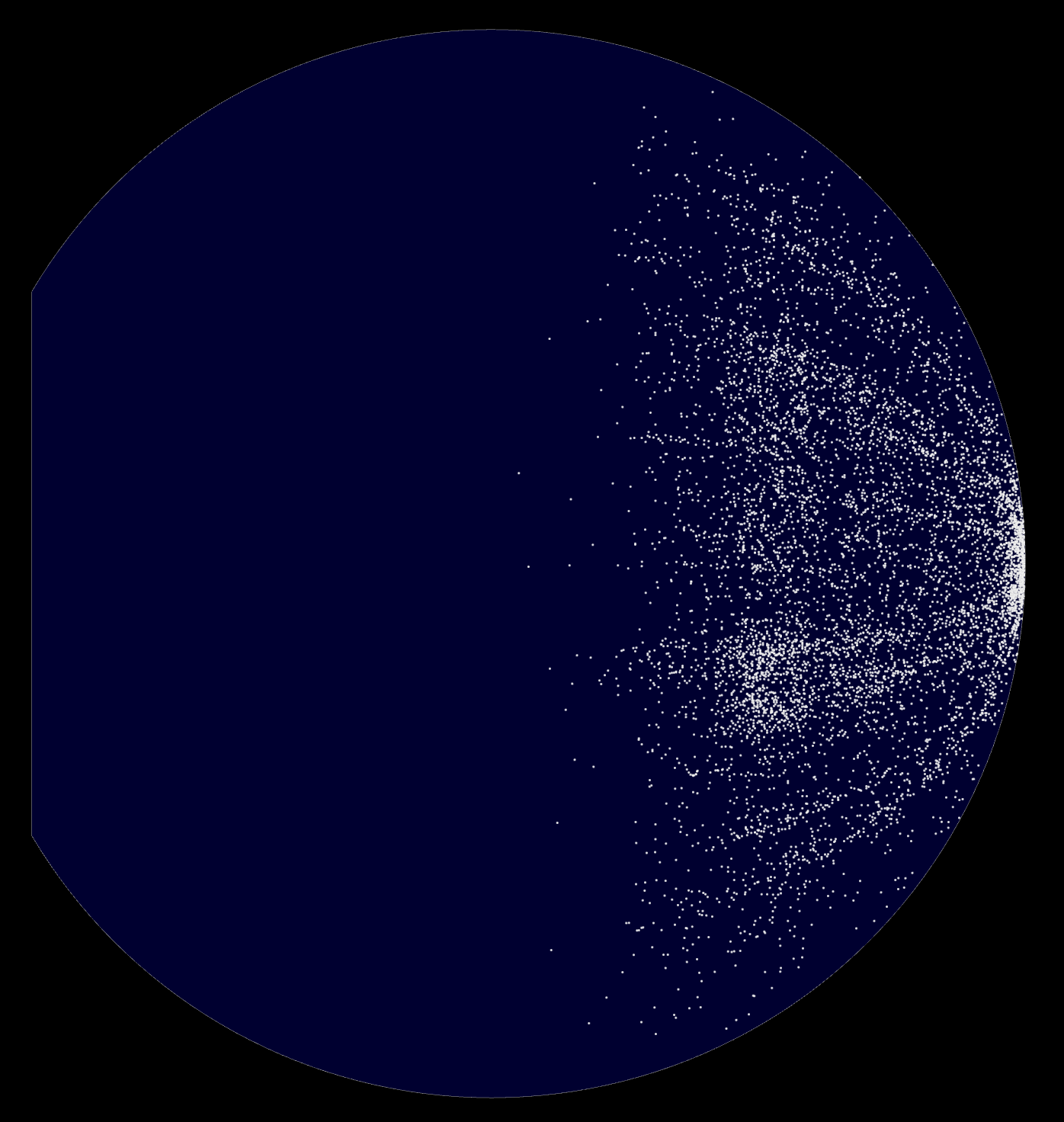
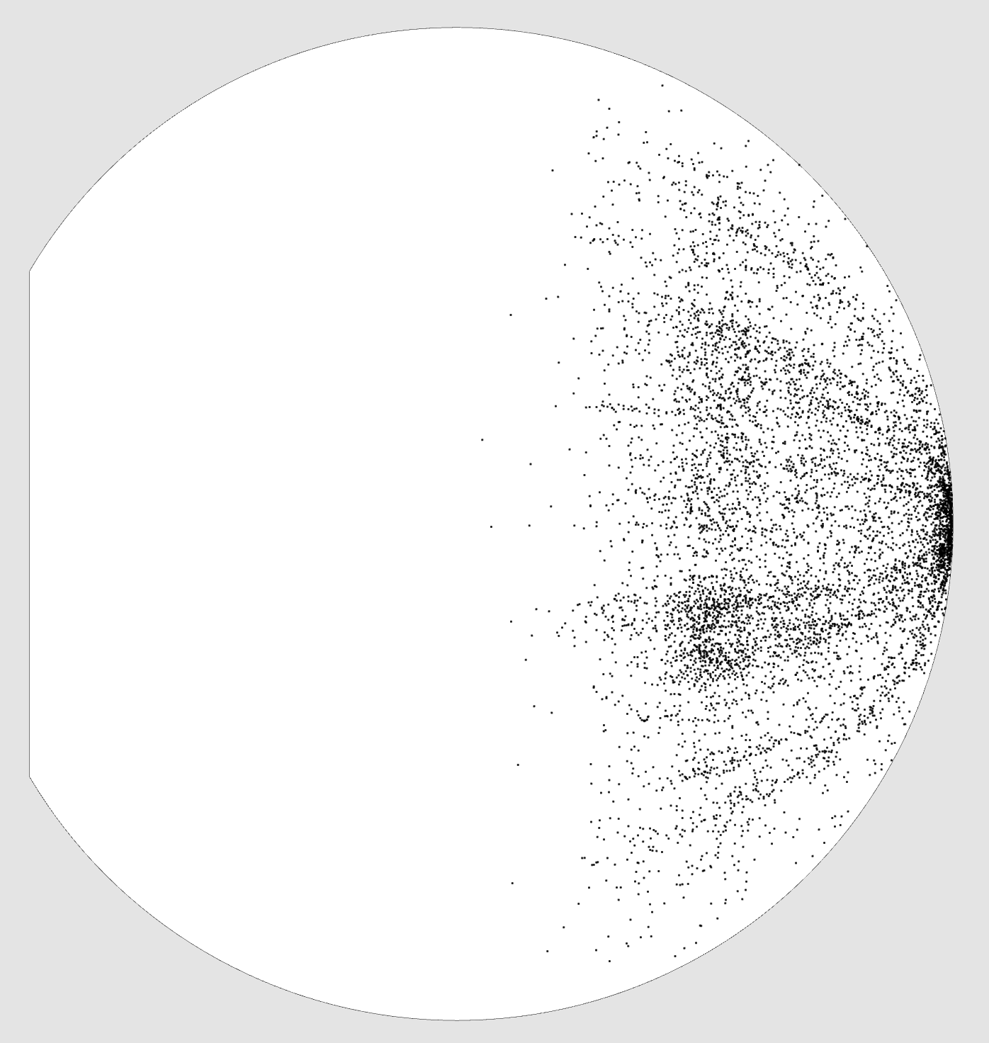Our galaxy is on the far right.

Edge view, negative curvature

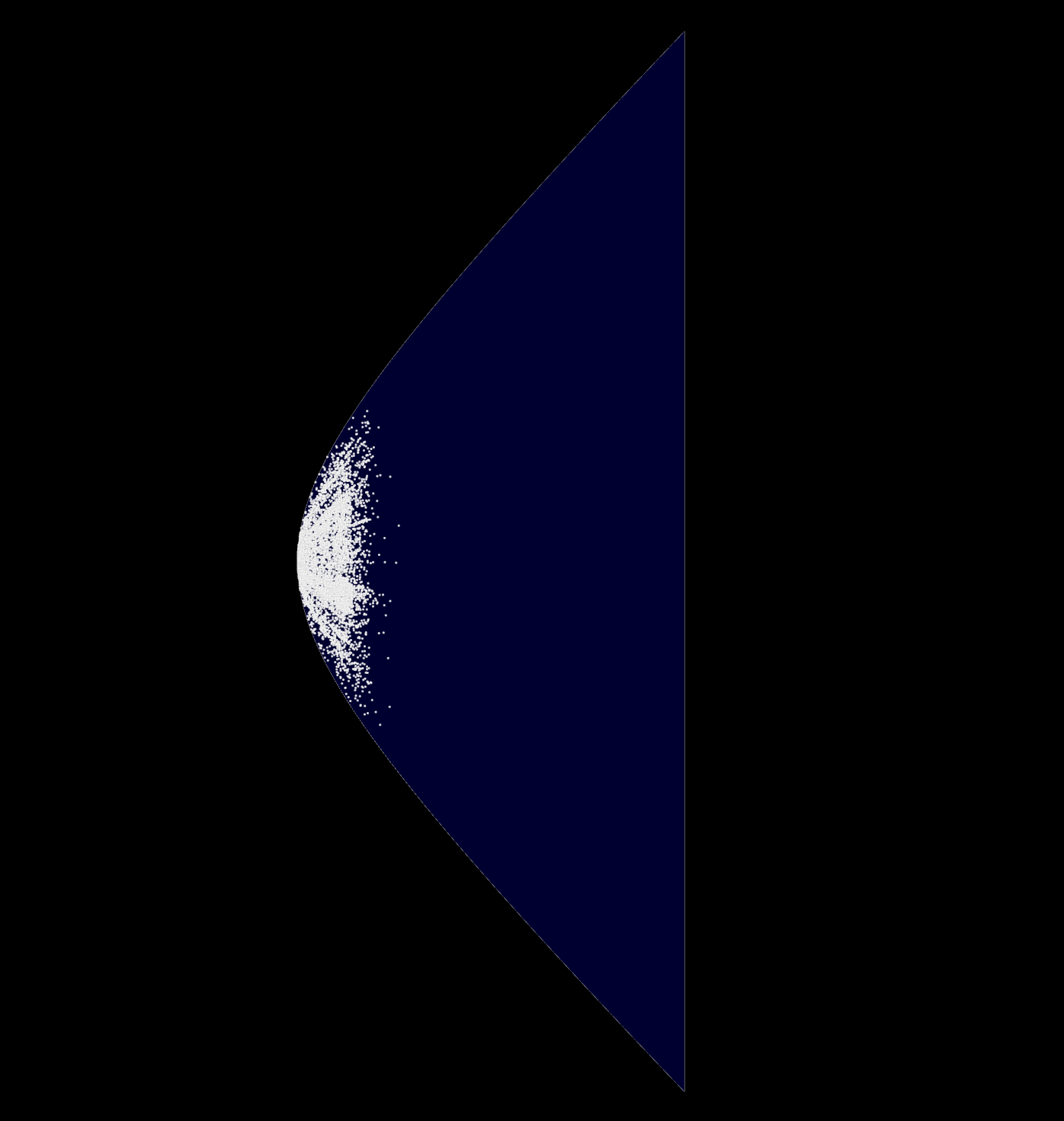
Our galaxy is on the far left.

Sky view

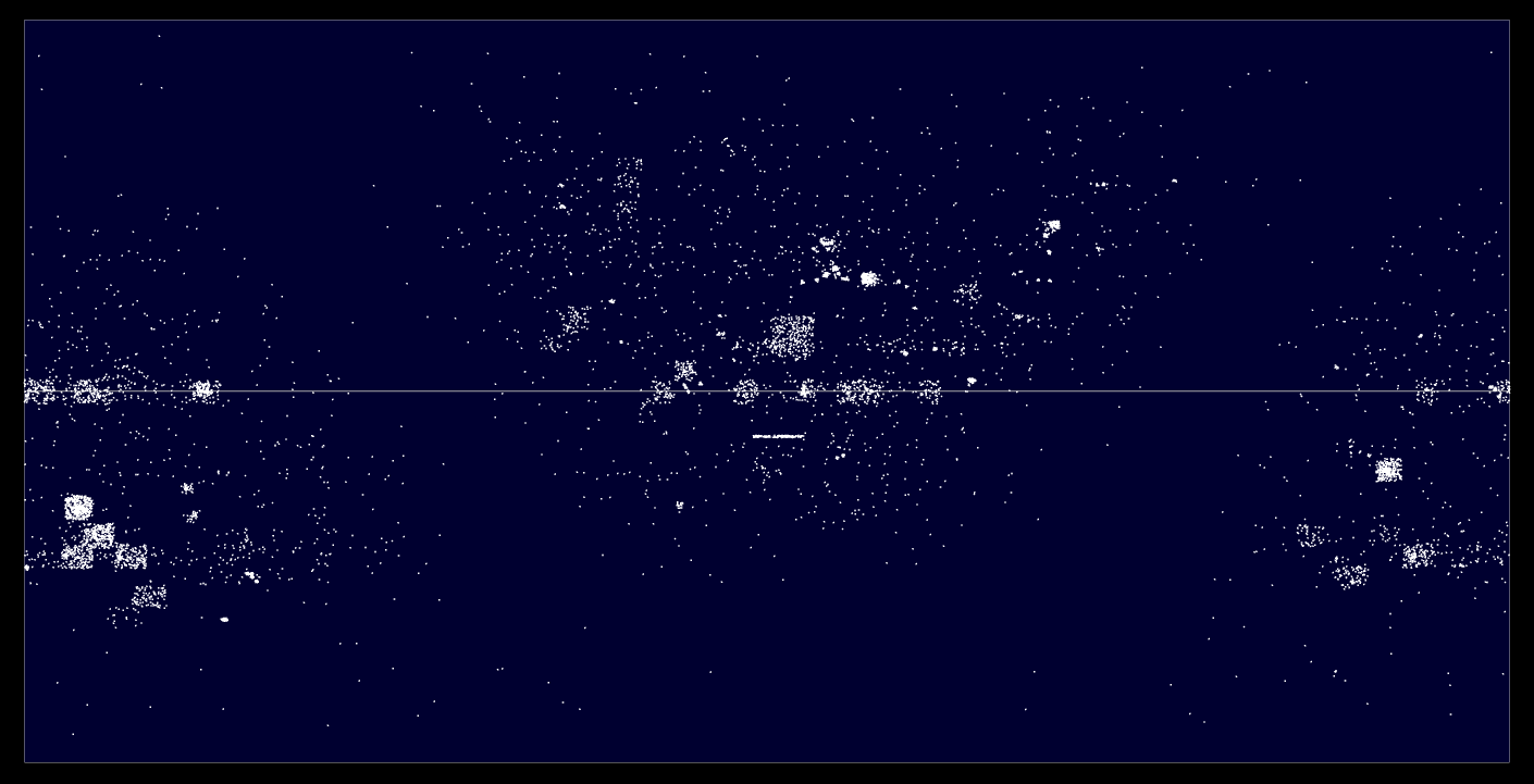
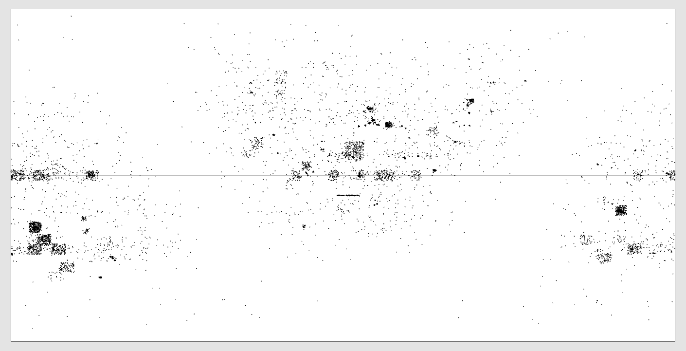Here we see what radio telescopes have observed from Earth.

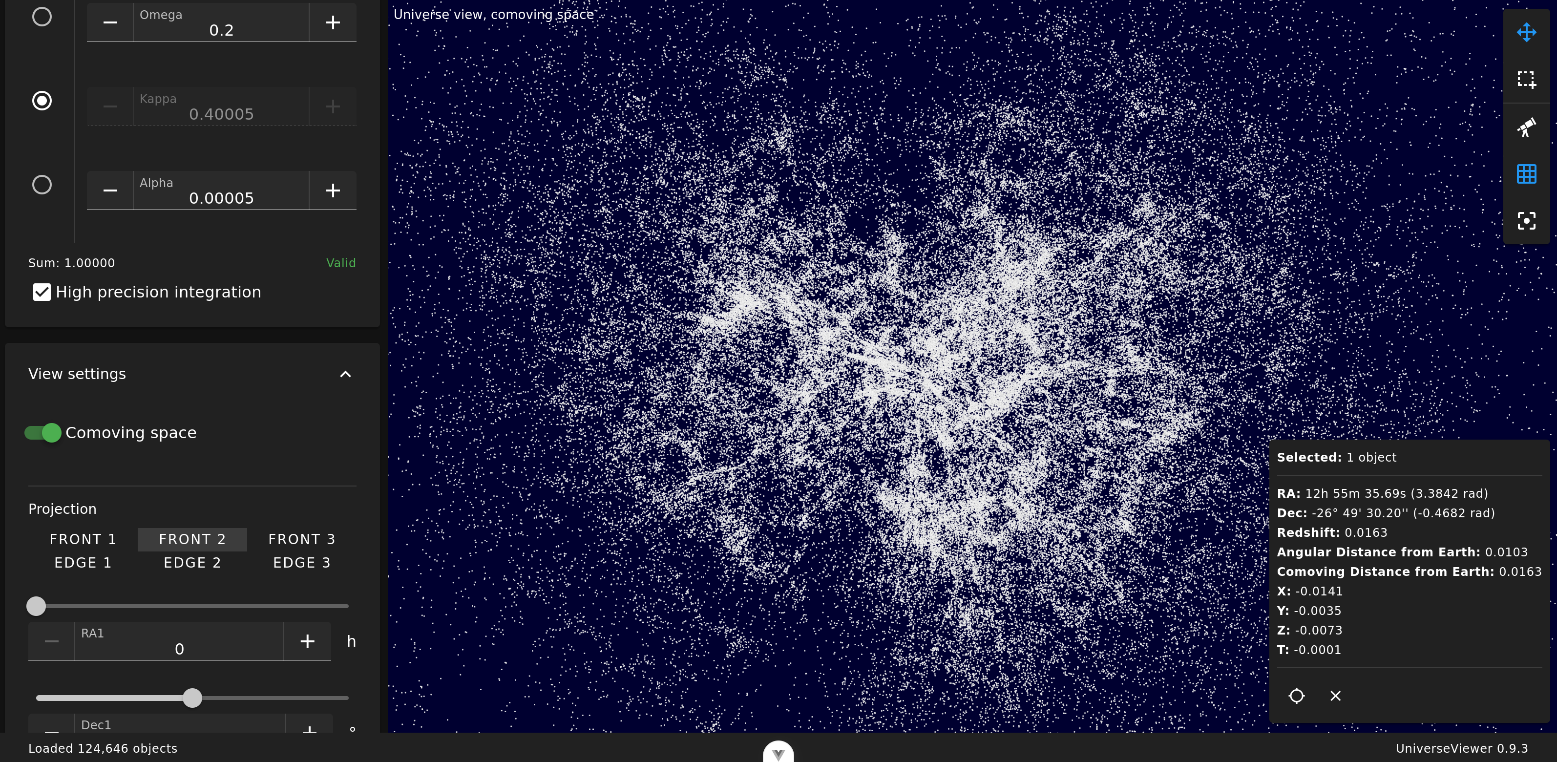
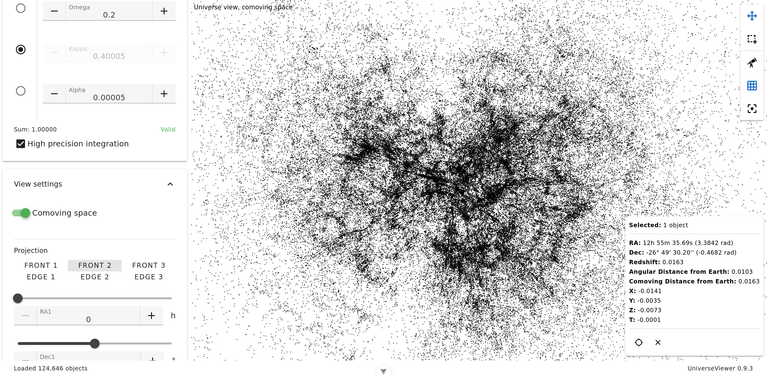
Objects selection

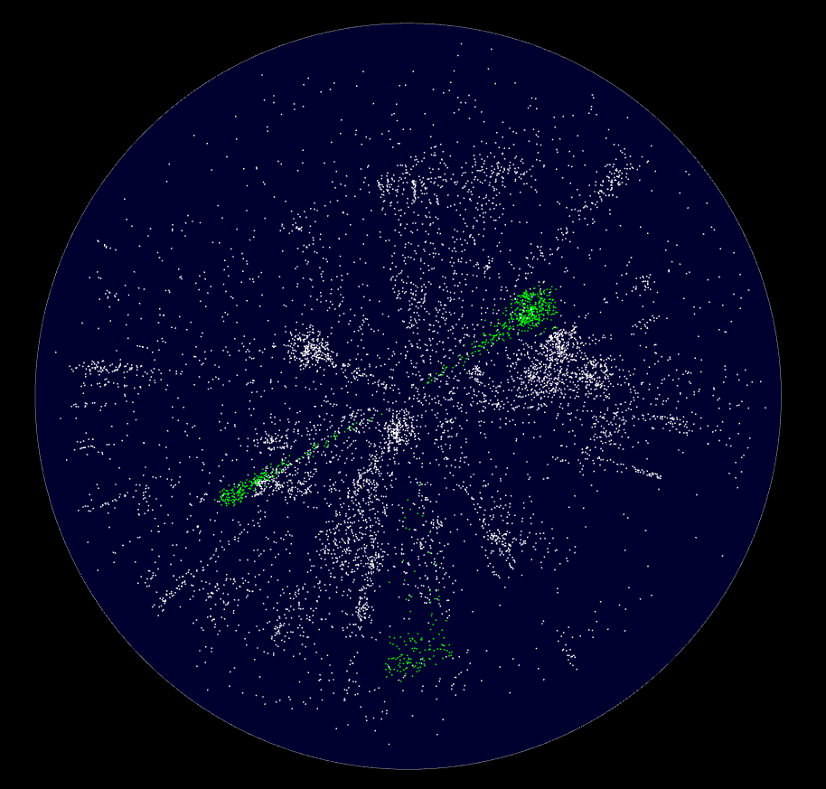
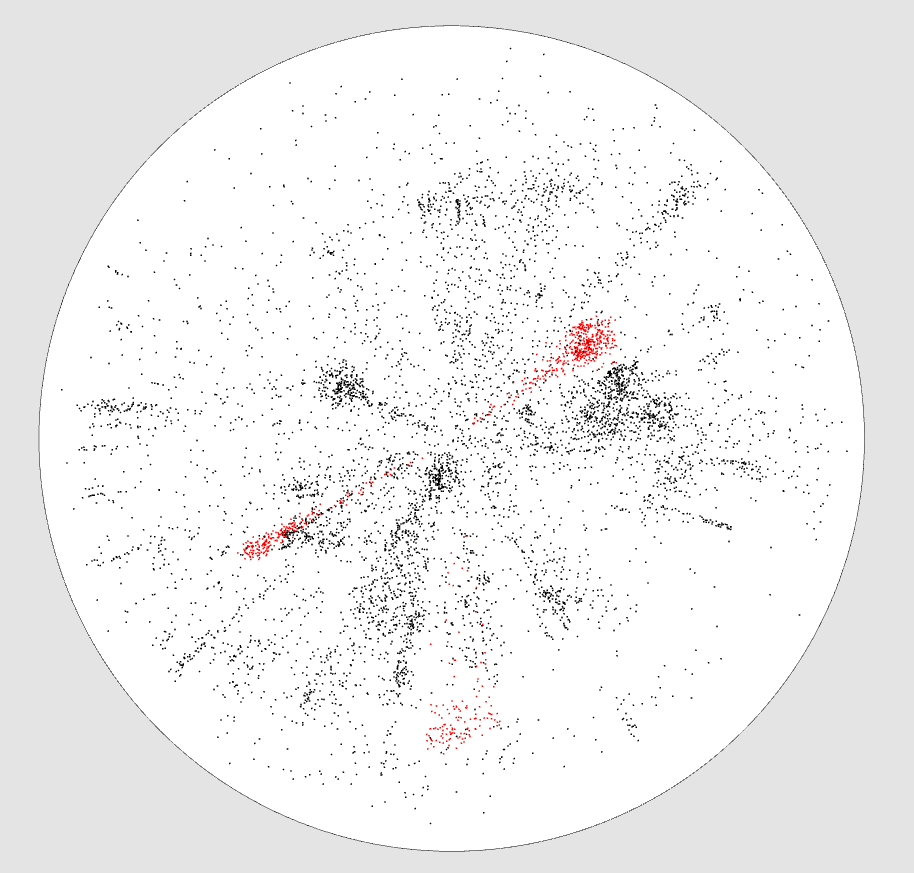You can select objects with an additive or intersection selection tool, allowing to accurately select areas from different views.

Selected objects are in green.

Selected objects are in red.

6dF Galaxy Survey

6dF Galaxy Survey catalog is composed of 124,646 objects.

Zoom

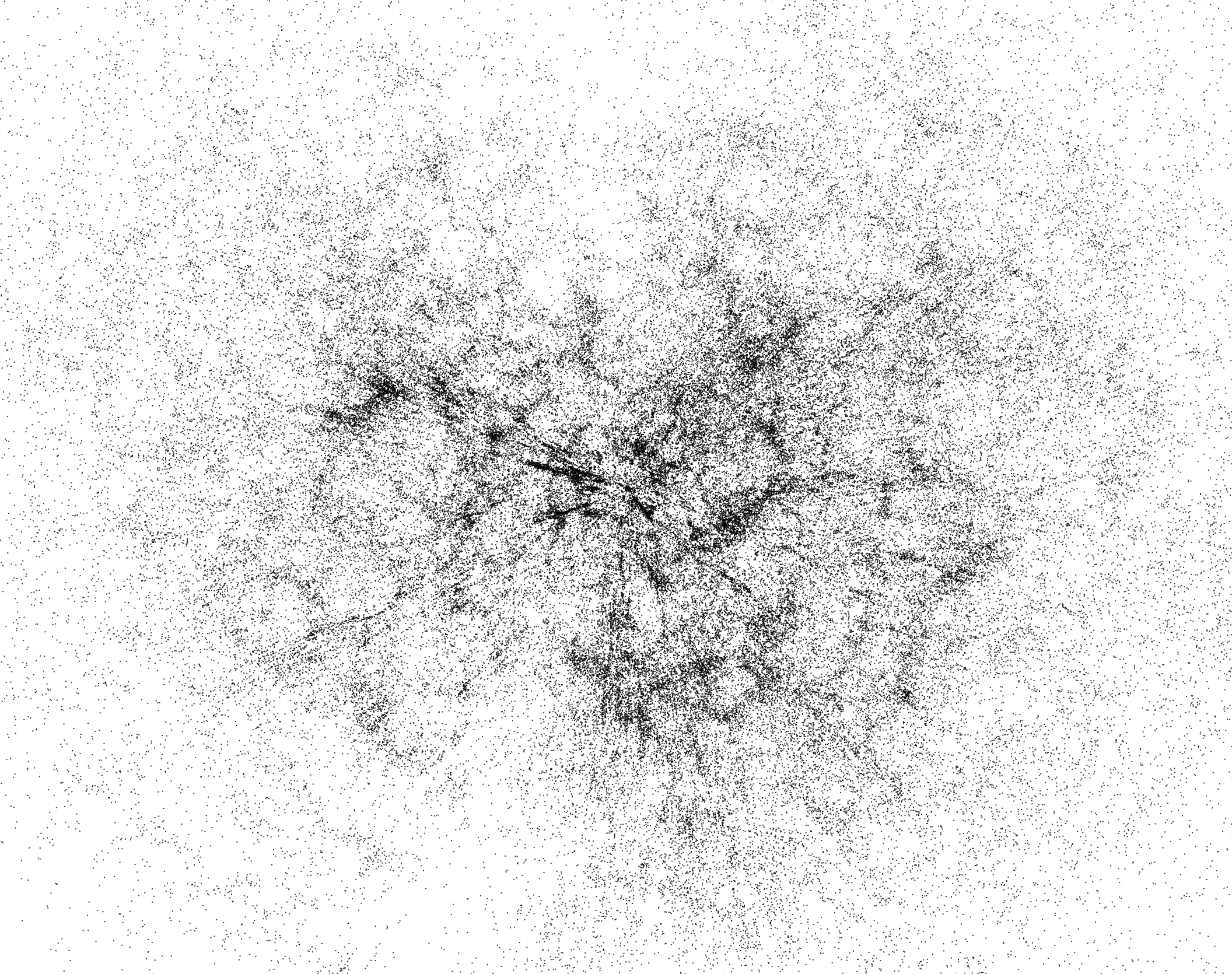
Here we are in face vue 2, and the projection is zoomed with our galaxy approximately in its center.

Quasars (13th Ed.) (Veron-Cetty+)

This catalog is composed of 133,335 objects.

Coloration en dégradé du redshift

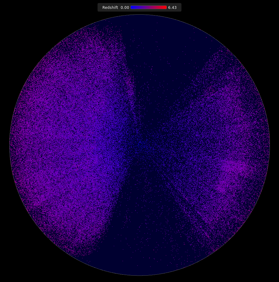
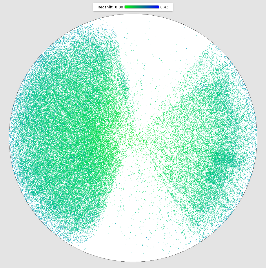
To better appreciate displayed objects redshift, it is possible to give them a color.

Nearest objects from our galaxy are in blue, most distant in red.

Nearest objects from our galaxy are in green, most distant in green.

Distance Between Two Objects

Let $x_1$ and $x_2$ be the directions on the sky of two objects. The apparent angular separation between them is given by:

$$\cos {\theta }_{12}=⟨x_1,x_2{⟩}_3$$

which can be written explicitly as:

$$\begin{array}{r}\cos {\theta }_{12}=\cos (R{A}_{obj1}-R{A}_{obj2})\cos (De{c}_{obj1})\cos (De{c}_{obj2})\\ +\sin (De{c}_{obj1})\sin (De{c}_{obj2})\end{array}$$

To compute the geodesic distance between these objects in a space with non‑zero curvature, two cases must be considered:

case $k_0>0$ (spherical geometry),

$$\begin{array}{l}\cos {\hat{\tau }}_{12}=\cos {\theta }_{12}\sin {\hat{\tau }}_1\sin {\hat{\tau }}_2+\cos {\hat{\tau }}_1\cos {\hat{\tau }}_2\\ {\hat{\tau }}_{12}=\arccos (\cos {\hat{\tau }}_{12}),\end{array}$$

case $k_0<0$ (hyperbolic geometry),

$$\begin{array}{l}\cosh {\hat{\tau }}_{12}=\cosh {\hat{\tau }}_1\cosh {\hat{\tau }}_2-\cos {\theta }_{12}\sinh {\hat{\tau }}_1\sinh {\hat{\tau }}_2\\ {\hat{\tau }}_{12}=\mathrm{arccosh}(\cosh {\hat{\tau }}_{12}),\end{array}$$

where ${\hat{\tau }}_1$ and ${\hat{\tau }}_2$ are the angular (geodesic) distances of the objects from the Earth.

The dimensionless comoving distance is then given by:

$${\tau }_{12}=\frac{{\hat{\tau }}_{12}}{\sqrt{|k_0|}}$$

In the special case of a flat space, the comoving distance is obtained using the Euclidean law of cosines:

$${\tau }_{12}=\sqrt{{\tau }_1^2+{\tau }_2^2-2{\tau }_1{\tau }_2\cos {\theta }_{12}},$$

Finally, the comoving distance can be expressed in physical units (Mpc) as:

$$r={\tau }_{12}\frac{c}{H_0}$$

where $c$ is the speed of light in km/s (299,792.458 km/s) and $H_0$ is the Hubble constant.

Implementation

Here are some technical choices regarding the implementation.

Integral computation

Two ways to compute integrals have been implemented:

• the Romberg method, fast but less accurate,
• the trapezoidal rule, slower but more precise.

Parallel processing

By default, in a web browser, JavaScript runs on the main thread, which also handles the page rendering code. Not only does this loop use only a single CPU core, but intensive computations also freeze the user interface.

We have a large number of objects for which we compute projections based on cosmological parameters. This set of objects can easily be split into several chunks so that processing can be done on multiple cores at the same time.

Parallelization in Universe Viewer uses web workers, which allow us to divide the workload according to the number of available CPU cores. This process is performed in the following files:

• workerPool.js, which manages the pool of workers, their lifecycle, and their execution for projection calculation,
• projectionWorker.js, the worker task code that processes a subset of the objects,
• projection.js, the projection computation functions.

If the number of objects to process falls below a certain threshold, the computation is not parallelized because the overhead caused by the workers management would be counterproductive.

To make the parallelisation more relevant, we are using shared memory between workers and graphical rendering, using SharedArrayBuffer: there is zero data copy since a catalog has been loaded.

If SharedArrayBuffer is unavailable, for example due to security constraint not met, computing is not parallelized.

These optimizations allow UniverseViewer to handle million targets catalogs, as AGN/QSO Value-Added Catalog for DESI DR1, or Million Quasars Catalog, Version 8.

---

Official Website
GitHub Page
Framework for cosmography at high redshift - R. Triay, L. Spinelli, R. Lafaye (1996), HTML version, et text PDF version
Romberg method for integral computation
Trapezoidal rule for integral computation
Old Java version